Voice-First Future: Lessons From Scaling Browser-Based Audio

Sound is a form of energy created by the vibration of a medium. The vibration creates a pressure wave that travels through the medium, be it air, water, or any other material, and that pressure wave is what we perceive as sound.

A Quick History of Audio

In the analog era, we captured sound physically. Now, in the digital age, we store it as numbers in bits and bytes.

Analog Sound

In the early days, audio recording relied on analog methods, such as magnetic tape and vinyl records. In analog recording, sound waves are converted into a continuous electrical signal. This signal is then physically imprinted onto a medium, like the grooves of a vinyl record. Playback reverses the process, converting the physical pattern back into an electrical signal and then into sound.

Take a vinyl record as an example: Sound waves are picked up by a microphone, which converts them into an electrical signal. This signal is then sent to a cutting lathe that physically engraves the sound wave’s pattern into the record’s surface, creating a continuous groove.

During playback, a turntable’s needle tracks this groove. Its vibrations are then converted back into an electrical signal by a phono cartridge. This electrical signal is amplified and finally sent to speakers, which transform it back into the sound we hear.

While the process of recording and playing back sound using analog methods was complex, it served for many years as the primary way to create and distribute music and other audio content.

Digital Sound

Analog sound, however, had its limitations. Recordings could degrade over time, and they weren’t easily portable. This is where digital audio revolutionized the field.

In the digital age, we capture sound as numerical data. Digital audio is a representation of sound that’s stored in a digital format. It’s created by taking rapid “snapshots” (sampling) of the sound wave at regular intervals and then converting those amplitude snapshots into a series of numbers. These numbers can then be efficiently stored, processed, and played back using various digital devices.

Digital audio first emerged in the 1960s with Bell Labs’ pioneering Digital Audio Tape (DAT). By 1979, Sony and Philips introduced the Compact Disc (CD) as the first commercially available digital audio system.

This shift profoundly changed how we create and consume sound, paving the way for MP3s, streaming services, and the advanced audio tools we use today.

Digital Audio 101: Sampling and Bits

Digital audio converts continuous waves into discrete data. Two key concepts come into play: sampling rate and bit depth.

Sampling Rate

Sampling rate is how often we “snapshot” the sound wave per second, measured in Hz. E.g., 44.1 kHz means 44,100 snapshots/second. This means that for each second of audio, there are 44,100 individual samples representing the amplitude of the sound wave at different points in time. Higher rates capture more detail but require more storage.

Why does this matter? Humans hear frequencies from about 20 Hz (deep bass) to 20 kHz (high treble). To capture a frequency accurately without distortion (aliasing), the Nyquist-Shannon theorem (https://en.wikipedia.org/wiki/Nyquist%E2%80%93Shannon_sampling_theorem) says we must sample at least twice that frequency.

Going by the Nyquist theorem, for full human hearing (up to 20 kHz), the minimum sampling rate needed is 40 kHz. CDs use 44.1 kHz for a safety margin and also to match 1970s video tech standards.

Bit Depth

Each sample measures the wave’s amplitude (height/loudness). Bit depth is how finely we measure it, like the number of colors in a photo.

16-bit: 65,536 possible values for amplitude.

24-bit: Over 16 million possible values.

In general, higher sampling rates and bit depths result in better audio quality, but they also require more storage space and processing power.

Audio in Browsers: The Web Audio API

Browsers capture audio using the device’s microphone and encode this signal into a digital format that can be processed and manipulated with JavaScript. The tool for this job is the Web Audio API.

The Web Audio API can feel complex, but its core idea is simple: it lets you build a flowchart for the sound. Think of it as a virtual sound studio inside the browser.

The AudioContext: The Virtual Studio

Everything in the Web Audio API happens inside an AudioContext. It’s the main object that manages all audio operations. You can’t play, process, or create sound without one. It builds and contains an audio processing graph, a term for the path the sound takes from its source to its destination.

The data flowing through this graph is typically raw PCM (Pulse Code Modulation) data represented as a Float32Array. In this format, each number in the array is a sample of the audio signal, with values ranging from -1.0 (minimum amplitude) to 1.0 (maximum amplitude). This high-precision, 32-bit floating-point format is excellent for processing but is different from the format our ASR systems expect, which sets up a key challenge we’ll address later.

The graph itself is made of audio nodes, which are the building blocks of your sound flowchart. Let’s look at the three main types of nodes:

Source Nodes: Where the sound comes from (e.g., a microphone or an audio file).

Processing Nodes: Nodes that modify the sound (e.g., changing volume, adding effects).

Destination Node: Where the sound ends up (usually, your speakers).

Example: Basic Audio Playback

Imagine you want to play an MP3 file in the browser. You wouldn’t just point to the file; you’d build a simple audio graph. The sound from the file is fed into a source node, which is then connected directly to the destination node (the speakers).

Example: Capturing Mic Audio with a Volume Knob

Let’s say you want to capture audio from a user’s microphone and make it louder. Here, the sound starts at the microphone, flows into a source node, passes through a processing node to adjust the volume, and finally goes to the destination node. The processing node we’d use is a GainNode, which acts just like a volume knob.

This node-based system is incredibly powerful. By connecting different types of nodes in various combinations, you can create complex audio effects, visualizations, and processing pipelines right in the browser.

ASR at Suki: 16kHz and beyond

For Automatic Speech Recognition (ASR) systems, audio quality is crucial. While browsers capture audio at a high-fidelity 44.1 kHz or 48 kHz, our ASR models are optimized specifically for speech.

Human speech primarily falls within a frequency range of 300 Hz to 3,400 Hz. Applying the Nyquist theorem, the minimum sampling rate required to capture this is about 6.8 kHz (3,400 Hz \* 2). But ASR systems typically use 8 kHz or 16 kHz, for various reasons, and one of them is compatibility with the existing standards and hardware.

8 kHz is the standard for “narrowband” audio, used in traditional landline telephony.

16 kHz is the standard for “wideband” or VoIP (Voice over IP) audio, offering higher quality.

For modern ASR, 16 kHz has become the sweet spot, providing excellent clarity for speech without unnecessary data.

The next one is bit depth. We need to choose a format that balances quality and efficiency.

Using 8-bit audio would result in a lower dynamic range and more noise, which could harm recognition accuracy.

Using 24-bit or 32-bit audio would create much larger files without a significant improvement for speech signals.

This makes 16-bit PCM the ideal choice. It provides a dynamic range of about 96 dB, which is more than enough to capture the nuances of human speech without bloating file sizes.

So, we have our target format: 16 kHz, 16-bit PCM audio. But we can’t just send a continuous stream to our backend. To balance latency and efficiency, we send the audio in small, regular packets. ASRs typically recommend a 100ms frame size, meaning we send 10 frames every second.

For a sampling rate of 16 kHz, each 100-ms frame contains 1,600 samples (16,000 samples/sec _ 0.1 sec). Since each sample is a 16-bit (2-byte) integer, each frame is 3,200 bytes (1,600 _ 2), or 3.2 KB.

Our challenge is now clear: take the high-quality 44.1 kHz/32-bit audio from the browser and efficiently convert it into a stream of 3.2 KB, 16 kHz/16-bit audio chunks to send to our ASR engine, all in real-time.

Suki’s Audio Capture Evolution: Our Story

Our audio system started simple and grew with Suki’s needs. Here’s how it evolved, phase by phase.

Phase 1: Starting with a Third-Party Solution

Initially, we used Picovoice’s (https://picovoice.ai/) open source library called Web Voice Processor (https://github.com/Picovoice/web-voice-processor), a battle-tested library that handled the complexity for us. It captured mic audio and automatically downsampled it to the 16 kHz/16-bit format we needed. This was a great starting point.

This worked well for us, but soon we discovered that if a user’s microphone was muted, we were still capturing, processing, and sending complete silence to our backend, which resulted in empty notes.

Phase 2: Adding Decibel Detection

To solve the “empty audio” problem, we added a decibel meter. This allowed us to monitor the audio level in real-time. If we detected prolonged silence, we could pause the session and alert the user to check their microphone or browser settings.

Phase 3 & 4: Unifying for Scale and Solving Race Conditions

As Suki expanded to new products like a Chrome extension and a Web SDK, having separate audio implementations became unmanageable. Every new change needed to be updated in multiple places. For this reason, we needed a unified, centralized audio package.

This rewrite helped us discover a tricky race condition that existed with our old approach, which caused note failures due to no audio being sent to the backend even though the session was going on.

Imagine two features both needing the microphone, like our “Suki Badge” and an “Ambient” session.

When a user starts an ambient session, the app hides the badge first and then begins the session. However, as part of the badge’s cleanup process, we rightfully stop the recording and release the AudioContext asynchronously. This creates a race condition: sometimes the badge releases the AudioContext after the ambient session has already acquired it and started recording. When this happens, the ambient session’s audio capture is abruptly terminated, resulting in no audio being sent to the backend.

This is a classic software engineering problem: managing safe access to a shared resource. In software architecture, a common solution is a mutex (mutual exclusion), which acts like a key to a room; only one process can hold the key at a time. A more robust approach is a centralized manager that owns the resource and fields requests.

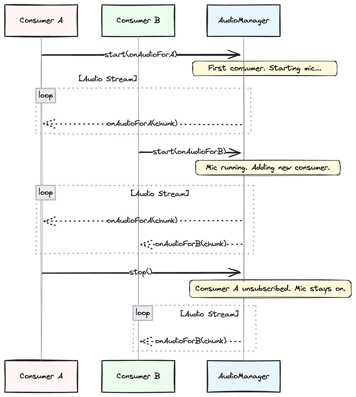
We chose a publish-subscribe (pub/sub) model, which is a sophisticated version of a centralized manager. It decouples our features (the “consumers”) from the audio system. The “Suki Badge” doesn’t need to know about the “Ambient” session; it just interacts with our central AudioManager.

This AudioManager is the core of our solution. Here’s how it works:

Consumers Subscribe: Any feature needing audio calls AudioManager.start(listener). The listener is a function that will receive audio chunks. The AudioManager adds this listener to a list of active subscribers.

Smart Resource Management: If start() is called and the microphone is already running, the AudioManager simply adds the new listener to its broadcast list. If the microphone is off, it initiates the audio capture first and then adds the listener.

Publishing Data: Once running, the AudioManager publishes audio chunks to all active listeners.

Graceful Unsubscribe: When a consumer is done, it calls AudioManager.stop(), and the AudioManager removes its listener. It only stops the microphone and releases the AudioContext when the very last listener has unsubscribed.

This way, consumers don’t have to worry about the underlying state. But even this system needs to handle near-simultaneous requests safely. To prevent race conditions when multiple consumers try to start or stop at once, the AudioManager uses an internal lock (a mutex) to ensure it only processes one of these subscription changes at a time. This makes each transition atomic: an all-or-nothing operation that keeps the audio logic stable.

Phase 5: Adding “Plug-and-Play” Voice Activity Detection (VAD)

As part of the “Badge state transitions” effort to improve Badge UX responding to commands, we introduced Voice Activity Detection (VAD), an on-device model that can distinguish human speech from silence or background noise.

However, integrating it introduced two major complexities.

First, the data format: Our pipeline was now standardized on producing Int16Array chunks for our backend. But the VAD model required the precision Float32Array. We couldn’t simply switch our entire pipeline, as the backend ASR still needed Int16Array

Second, VAD wasn’t needed everywhere. We only wanted this extra processing for voice commands. So it needed to be a “plug-and-play” component.

Finally, to ensure a snappy user experience on the web, we couldn’t afford to download and initialize the VAD model every time the app is loaded, because the file size is huge. So we implemented a caching strategy to fetch the ONNX model only once and reuse it every time.

Phase 6: The Telehealth Overhaul & The Final Architecture

Our biggest challenge and a complete rewrite came with the Telehealth use case. For our Chrome extension, we needed to capture audio from two sources simultaneously: the doctor’s microphone and the patient’s audio from the Telehealth browser tab. This meant sunsetting our Picovoice dependency and building our own pipeline from scratch.

This was a major undertaking, especially since our audio library is a shared package. The new, more complex telehealth capture logic had to be implemented carefully so it would only activate when running inside the extension, leaving other products unaffected.

Challenge 1: Mixing Two Streams — Like a Sound Engineer

Imagine you’re the sound engineer at a concert with two performers: a singer (the doctor) and a guitarist (the patient). Both have their own microphones, and your job is to make sure the audience hears both of them clearly through the main speakers. You’d use a mixing board.

• The Inputs: The doctor’s audio is one input, and the patient’s audio is another. In our code, useMicrophoneAudioCapture and useTabAudioCapture are like setting up these individual microphones.
• The Volume Sliders: On the mixing board, each mic has its own volume slider. In the Web Audio API, this is a GainNode. We give one to each audio source.
• The Main Output: All sound is funneled into a single main output. This is our MediaStreamAudioDestinationNode, which combines everything into one perfectly mixed track.

Challenge 2: The Downsampling and the Firefox compatibility

With Picovoice gone, the job of downsampling from the browser’s native 44.1/48 kHz to our required 16 kHz fell to us. Our initial plan to simply request 16 kHz from the browser while creating an AudioContext failed when we discovered Firefox ignored the request. We had to build our own high-quality resampler.

const audioContext = new AudioContext({ samplingRate: 16000 }) // ignored by firefox

Our Solution: AudioWorklet

The main browser thread is busy handling everything you see and click on the user interface. If we tried to do intense audio processing there, the entire page would stutter and freeze. An AudioWorklet is a special kind of script that runs on its own, separate, high-performance thread. It’s designed specifically for this kind of heavy lifting, ensuring the app stays responsive.

The single, mixed stream from our “virtual mixer” was piped into this worklet, which then became a multi-stage factory for our audio:

1. Buffering the Stream: Audio data doesn’t arrive in little packages; it’s a continuous stream. To manage this, we implemented a Ring Buffer. Think of it as a temporary holding area. It gives our worklet a small, predictable buffer of audio to work with, ensuring we don’t drop any data while we’re busy with the next steps.
2. Custom Resampling: For every block of high-resolution audio that comes off the buffer (e.g., 48,000 samples per second), our custom algorithm intelligently calculates a new, smaller set of samples to create a clean 16,000 samples-per-second stream.
3. Hand-rolled Volume Normalization: Picovoice helped us detect silence, and with it removed, we needed a custom solution to replace it. Custom signal processing algorithms provided a more reliable solution than even Picovoice could provide.
4. Final Format Conversion: As the very last step, the worklet takes the processed high-precision decimal 16 kHz data stream into a simpler, compliant format.

Once this final conversion is done, the worklet posts the finished audio chunk back to our AudioManager on the main thread, which then publishes it to all active consumers.

This brings us to our final architecture, which handles multiple consumers, different capture modes, and optional processing steps, all orchestrated by the AudioManager.

Phase 7: Looking Ahead

Our latest evolution is a new, framework-agnostic core audio library. By decoupling our audio logic from any specific UI framework like React, we can now support any future products that may use different JavaScript frameworks.

But that’s a story of architectural decisions, dependency management, and engineering solutions that deserves its own deep dive.

By the Numbers: A Quick Stats Breakdown

• Our Target Format: 16 kHz, 16-bit PCM audio.
• Streaming Cadence: We send audio to our backend in chunks every 100 milliseconds (that’s 10 chunks per second).
• Chunk Size: Each 100-ms chunk contains 1,600 audio samples and has a size of 3.2 KB.
• Data Rate: This works out to a steady stream of 32 KB per second.

Total Data Size (Mono):

• A 10-minute session generates about 18.75 MB of audio data.
• A 60-minute session generates about 112.5 MB of audio data.
• The calculation is straightforward: (Total Seconds) * (32 KB/second) / (1024 KB/MB). For 10 minutes, that’s 600 * 32 / 1024 = 18.75 MB.

Conclusion

In this blog post, I simplified certain concepts and technical details to provide a high-level overview of how audio works in browsers and the challenges we encountered along the way. I hope this has given you a clearer understanding of the intricacies involved in building and processing audio in web applications.

As our products continue to evolve, we remain focused on improving the performance, reliability, and overall user experience of our audio capture mechanisms. This is an ongoing effort, shaped by lessons learned and the feedback we gather from real-world usage.

The audio library itself has grown and matured over time through the collective efforts of many. There is no single author to credit. I’d like to acknowledge the Suki Engineering and QA Automation teams for their invaluable contributions in building the library, identifying issues such as empty notes, performing thorough code reviews, and carrying out relentless regression testing across products to ensure its reliability and performance.